Machine Learning Part-01

Linear Regression Example

Implement Linear Regression for Boston House Price Problem

1
2
3
4
5
6
7
8
9
import random

import pandas as pd
import matplotlib.pyplot as plt
import seaborn as sns
import numpy as np
from sklearn.datasets import load_boston
from matplotlib.animation import FuncAnimation
import re

Part-01: Linear Regression

1
2
3
4
5
6
7
8
9
10
11
12
13
14
15
16
17
18
19
20
21
22
23
24
25
26
27
28
29
30
31
32
33
34
35
36
37
38
39
40
41
42
43
44
45
46
47
48
49
50
51
52
53
54
55
56
57
58
59
60
61
62
63
64
65
66
67
68
69
70
71
72
73
74
75
76
77
78
79
80
81
82
83
84
85
86
87
88
89
90
91
92
93
94
95
96
97
98
99
100
101
102
103
104
105
106
107
108
109
110
111
112
113
114
115
116
117
118
119
120
121
122
123
124
125
126
127
128
129
130
131
132
133
134
135
136
137
138
139
140
141
142
143
144
145
146
147
148
149
150
151
152
153
154
155
156
157
158
159
160
161
162
163
164
165
166
167
168
169
170
171
172
173
174
175
176
177
178
179
180
181
182
183
184
185
186
187
188
189
190
191
192
193
194
195
196
197
198
199
200
housing_price = load_boston()
dataframe = pd.DataFrame(housing_price['data'])
dataframe.columns = housing_price['feature_names']
dataframe['price'] = housing_price['target']

# sns.heatmap(dataframe.corr(), annot=True, fmt='.1f')
# plt.show()

print(dataframe.columns)


"""
Index(['CRIM', 'ZN', 'INDUS', 'CHAS', 'NOX', 'RM', 'AGE', 'DIS', 'RAD', 'TAX',
'PTRATIO', 'B', 'LSTAT', 'price'],
dtype='object')
"""

rm = dataframe['RM']
lst = dataframe['LSTAT']
target = dataframe['price']

def model(x, w, b):
return np.dot(x, w.T) + b


def loss(yhat, y):
return np.mean( (yhat - y) ** 2)


def partial_w(x1, x2, y, yhat):
return np.array([2 *np.mean((yhat - y) * x1), 2 * np.mean((yhat - y) * x2)])


def partial_b(x1, x2, y, yhat):
return 2 * np.mean((yhat - y))

w = np.random.random_sample((1, 2))
print(w)
b = 0
alpha = 1e-5

epoch = 200
history = []

history_k_b_loss = []


"""
[[0.76646144 0.3095512 ]]
"""

for e in range(epoch):
losses = []
for batch in range(len(rm)):
random_index = random.choice(range(len(rm)))

x1, x2 = rm[random_index], lst[random_index]
y = target[random_index]

yhat = model(np.array([x1, x2]), w, b)
loss_v = loss(yhat, y)

w = w - partial_w(x1, x2, y, yhat) * alpha
b = b - partial_b(x1, x2, y, yhat) * alpha

losses.append(loss_v)

history_k_b_loss.append((w, b, loss_v))

if batch % 100 == 0:
print('Epoch: {}, Batch: {}, loss: {}'.format(e, batch, np.mean(losses)))

history.append(np.mean(losses))


"""
Epoch: 0, Batch: 0, loss: 151.86271856102778
Epoch: 0, Batch: 100, loss: 263.5872813250959
show more (open the raw output data in a text editor) ...

Epoch: 199, Batch: 500, loss: 28.308274447364248
"""
````


## Logstic Regression

```python
housing_price = load_boston()
dataframe = pd.DataFrame(housing_price['data'])
dataframe.columns = housing_price['feature_names']
dataframe['price'] = housing_price['target']

rm = dataframe['RM']
lst = dataframe['LSTAT']
price = dataframe['price']
print(np.percentile(price, 66))


"""
23.53
"""

# plt.hist(target)
# plt.show()

dataframe['expensive'] = dataframe['price'].apply(lambda p: int(p > np.percentile(price, 66)))
expensive = dataframe['expensive']

# print(dataframe.head())
print(dataframe['expensive'])


"""
0 1
1 0
..
505 0
Name: expensive, Length: 506, dtype: int64
"""

def logistic(x):
return 1 / (1 + np.exp(-x))


def model(x, w, b):
return logistic(np.dot(x, w.T) + b)


def loss(yhat, y):
return -1 * np.sum(y*np.log(yhat) + (1 - y) * np.log(1 - yhat))


def partial_w(x1, x2, y, yhat):
return np.array([np.sum((yhat - y) * x1), np.sum((yhat - y) * x2)])


def partial_b(x1, x2, y, yhat):
return np.sum(yhat - y)

w = np.random.random_sample((1, 2))
print(w)


"""
[[0.69565948 0.90768813]]
"""

b = 0
alpha = 1e-5

epoch = 200
history = []
history_k_b_loss = []

for e in range(epoch):
losses = []
for batch in range(len(rm)):
random_index = random.choice(range(len(rm)))

x1, x2 = rm[random_index], lst[random_index]
y = expensive[random_index]

yhat = model(np.array([x1, x2]), w, b)
loss_v = loss(yhat, y)

w = w - partial_w(x1, x2, y, yhat) * alpha
b = b - partial_b(x1, x2, y, yhat) * alpha

losses.append(loss_v)

history_k_b_loss.append((w, b, loss_v))

if batch % 100 == 0:
print('Epoch: {}, Batch: {}, loss: {}'.format(e, batch, np.mean(losses)))

history.append(np.mean(losses))


"""
Epoch: 0, Batch: 0, loss: 3.14765267665445e-06
Epoch: 0, Batch: 100, loss: 13.555508645878497
show more (open the raw output data in a text editor) ...

Epoch: 199, Batch: 500, loss: 0.31372698791846687
"""

predicated = [model(np.array([x1, x2]), w, b) for x1, x2 in zip(rm, lst)]
true = expensive

def accuracy(y, yhat):
return sum(1 if i == j else 0 for i, j in zip(y, yhat)) / len(y)

print(accuracy(true, predicated))


"""
0.0
"""

decision boundary

Linear Regression: Regression is implemented, including the definition of linear functions, why use linear functions, the meaning of loss, the meaning of gradient descent, stochastic gradient descent Use Boston house price dataset. The data set of Beijing housing prices in 2020, why didn’t I use the data set of Beijing housing prices? Boston: room size, subway, highway, crime rate have a more obvious relationship, so it is easier to observe the relationship Beijing's housing prices:! Far and near! Room Condition ==》 School District! ! ! ! => Very expensive Haidian District

1
2
3
4
5
6
7
8
9
10
11
12
13
14
15
16
17
18
19
20
21
22
23
24
25
26
27
28
29
30
31
32
33
34
35
36
37
38
39
40
41
42
43
44
45
46
47
48
49
50
51
52
53
54
55
56
57
58
59
60
61
62
63
64
65
66
67
68
69
70
71
72
73
74
75
76
77
78
79
80
81
82
83
84
85
86
87
88
89
90
91
92
93
94
95
96
97
98
99
100
101
102
103
104
import random

import numpy as np
import pandas as pd
from sklearn.datasets import load_boston

dataset = load_boston()
data = dataset['data']
target = dataset['target']
columns = dataset['feature_names']

dataframe = pd.DataFrame(data)
dataframe.columns = columns
dataframe['price'] = target

# print(dataframe.corr()) # show the correlation of dataframe variables
# correlation => If one value increases, it will cause another value to increase, and the correlation coefficient is closer to 1 if it increases in a certain proportion.
# correlation => 0 means there is no relationship between the two
# correlation => -1 One value increases, the other value must decrease, and the decrease is in equal proportion

# sns.heatmap(dataframe.corr())
# plt.show()

# RM: The average number of bedrooms in the community
# LSTAT: Percentage of low-income people around

rm = dataframe['RM']
lstat = dataframe['LSTAT']

def linear(x, w, b):
# vectorized model
return np.dot(x, w.T) + b


def loss(yhat, y):
# numpy broadcast numpy 广播方法
return np.mean( (yhat - y) ** 2)


def partial_w(x, y, yhat):
return np.array([2 * np.mean((yhat - y) * x[0]), 2 * np.mean((yhat - y) * x[1])])


def partial_b(x, y, yhat):
return 2 * np.mean((yhat - y))


def optimize(w, b, x, y, yhat, pw, pb, learning_rate):
w = w + -1 * pw(x, y, yhat) * learning_rate
b = b + -1 * pb(x, y, yhat) * learning_rate

return w, b

def train(model_to_be_train, target, loss, pw, pb):

w = np.random.random_sample((1, 2)) # w normal
b = np.random.random() # 0 深度学习的时候会和大家详细解释
learning_rate = 1e-5
epoch = 200
losses = []

for i in range(epoch):
batch_loss = []
for batch in range(len(rm)):
# batch training
index = random.choice(range(len(rm)))
rm_x, lstat_x = rm[index], lstat[index]
x = np.array([rm_x, lstat_x])
y = target[index]

yhat = model_to_be_train(x, w, b)
loss_v = loss(yhat, y)

batch_loss.append(loss_v)

w, b = optimize(w, b, x, y, yhat, pw, pb, learning_rate)

if batch % 100 == 0:
print('Epoch: {} Batch: {}, loss: {}'.format(i, batch, loss_v))
losses.append(np.mean(batch_loss))

return model_to_be_train, w, b, losses

if __name__ == "__main__":
import matplotlib.pyplot as plt

target = dataframe['price']

model, w, b, losses = train(linear, target, loss, partial_w, partial_b)
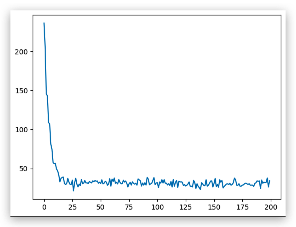
plt.plot(losses)
predicate = model(np.array([19, 7]), w, b)
print(predicate)

plt.show()


"""
Epoch: 0 Batch: 0, loss: 165.0318036522631
Epoch: 0 Batch: 100, loss: 1936.2111196826459
show more (open the raw output data in a text editor) ...

Epoch: 199 Batch: 500, loss: 0.024829543832110872
[88.74340551]
"""

image-20210831104443642

Logstic Regression

Linear Regression: Regression is implemented, including the definition of linear functions, why use linear functions, the meaning of loss, the meaning of gradient descent, stochastic gradient descent Use Boston house price dataset. The data set of Beijing housing prices in 2020, why didn’t I use the data set of Beijing housing prices? Boston: room size, subway, highway, crime rate have a more obvious relationship, so it is easier to observe the relationship Beijing's housing prices:! Far and near! Room Condition ==》 School District! ! ! ! => Very expensive Haidian District Harder than deep learning:

   1. compiler
   2. programming language & automata
   3. computer graphic
   4. complexity system
   5. computing complexity
   6. operating system
1
2
3
4
5
6
7
8
9
10
11
12
13
14
15
16
17
18
19
20
21
22
23
24
25
26
27
28
29
30
31
32
33
34
35
36
37
38
39
40
41
42
43
44
45
46
47
48
49
50
51
52
53
54
55
56
57
58
59
60
61
62
63
64
65
66
67
68
69
70
71
72
73
74
75
76
77
78
79
80
81
82
83
84
85
86
87
88
89
90
91
92
93
94
95
96
97
98
99
100
101
102
103
104
105
106
107
108
109
110
111
112
113
114
115
116
117
118
119
120
121
122
123
124
125
126
127
128
129
130
from sklearn.datasets import load_boston
import pandas as pd
import numpy as np

dataset = load_boston()
data = dataset['data']
target = dataset['target']
columns = dataset['feature_names']

dataframe = pd.DataFrame(data)
dataframe.columns = columns
dataframe['price'] = target

# print(dataframe.corr()) # show the correlation of dataframe variables
# correlation => If one value increases, it will cause another value to increase, and the correlation coefficient is closer to 1 if it increases in a certain proportion.
# correlation => 0 means there is no relationship between the two
# correlation => -1 One value increases, the other value must decrease, and the decrease is in equal proportion

# sns.heatmap(dataframe.corr())
# plt.show()

# RM: The average number of bedrooms in the community
# LSTAT: Percentage of low-income people around

rm = dataframe['RM']
lstat = dataframe['LSTAT']
price = dataframe['price']
greater_then_most = np.percentile(price, 66)
dataframe['expensive'] = dataframe['price'].apply(lambda p: int(p> greater_then_most))
target = dataframe['expensive']

print(dataframe[:20])


"""
CRIM ZN INDUS CHAS NOX RM AGE DIS RAD TAX \
0 0.00632 18.0 2.31 0.0 0.538 6.575 65.2 4.0900 1.0 296.0
1 0.02731 0.0 7.07 0.0 0.469 6.421 78.9 4.9671 2.0 242.0
2 0.02729 0.0 7.07 0.0 0.469 7.185 61.1 4.9671 2.0 242.0
3 0.03237 0.0 2.18 0.0 0.458 6.998 45.8 6.0622 3.0 222.0
4 0.06905 0.0 2.18 0.0 0.458 7.147 54.2 6.0622 3.0 222.0
5 0.02985 0.0 2.18 0.0 0.458 6.430 58.7 6.0622 3.0 222.0
6 0.08829 12.5 7.87 0.0 0.524 6.012 66.6 5.5605 5.0 311.0
7 0.14455 12.5 7.87 0.0 0.524 6.172 96.1 5.9505 5.0 311.0
8 0.21124 12.5 7.87 0.0 0.524 5.631 100.0 6.0821 5.0 311.0
9 0.17004 12.5 7.87 0.0 0.524 6.004 85.9 6.5921 5.0 311.0
10 0.22489 12.5 7.87 0.0 0.524 6.377 94.3 6.3467 5.0 311.0
11 0.11747 12.5 7.87 0.0 0.524 6.009 82.9 6.2267 5.0 311.0
12 0.09378 12.5 7.87 0.0 0.524 5.889 39.0 5.4509 5.0 311.0
13 0.62976 0.0 8.14 0.0 0.538 5.949 61.8 4.7075 4.0 307.0
14 0.63796 0.0 8.14 0.0 0.538 6.096 84.5 4.4619 4.0 307.0
15 0.62739 0.0 8.14 0.0 0.538 5.834 56.5 4.4986 4.0 307.0
16 1.05393 0.0 8.14 0.0 0.538 5.935 29.3 4.4986 4.0 307.0
17 0.78420 0.0 8.14 0.0 0.538 5.990 81.7 4.2579 4.0 307.0
18 0.80271 0.0 8.14 0.0 0.538 5.456 36.6 3.7965 4.0 307.0
19 0.72580 0.0 8.14 0.0 0.538 5.727 69.5 3.7965 4.0 307.0

PTRATIO B LSTAT price expensive
0 15.3 396.90 4.98 24.0 1
1 17.8 396.90 9.14 21.6 0
2 17.8 392.83 4.03 34.7 1
3 18.7 394.63 2.94 33.4 1
4 18.7 396.90 5.33 36.2 1
5 18.7 394.12 5.21 28.7 1
6 15.2 395.60 12.43 22.9 0
7 15.2 396.90 19.15 27.1 1
8 15.2 386.63 29.93 16.5 0
9 15.2 386.71 17.10 18.9 0
10 15.2 392.52 20.45 15.0 0
11 15.2 396.90 13.27 18.9 0
12 15.2 390.50 15.71 21.7 0
13 21.0 396.90 8.26 20.4 0
14 21.0 380.02 10.26 18.2 0
15 21.0 395.62 8.47 19.9 0
16 21.0 386.85 6.58 23.1 0
17 21.0 386.75 14.67 17.5 0
18 21.0 288.99 11.69 20.2 0
19 21.0 390.95 11.28 18.2 0
"""


def sigmoid(x):
return 1 / (1 + np.exp(-x))


def model(x, w, b):
return sigmoid(np.dot(x, w.T) + b)


def loss(yhat, y):
return -np.sum(y*np.log(yhat) + (1 - y)*np.log(1 - yhat))


def partial_w(x, y, yhat):
return np.array([np.sum((yhat - y) * x[0]), np.sum((yhat - y) * x[1])])


def partial_b(x, y, yhat):
return np.sum((yhat - y))


model, w, b, losses = train(model, target,loss, partial_w, partial_b)

random_test_indices = np.random.choice(range(len(rm)), size=100)
decision_boundary = 0.5


"""
Epoch: 0 Batch: 0, loss: 5.380792320433632
Epoch: 0 Batch: 100, loss: 4.821708458450062
show more (open the raw output data in a text editor) ...

Epoch: 199 Batch: 500, loss: 0.052809537616594626
"""

for i in random_test_indices:
x1, x2, y = rm[i], lstat[i], target[i]
predicate = model(np.array([x1, x2]), w, b)
predicate_label = int(predicate > decision_boundary)

print('RM: {}, LSTAT: {}, EXPENSIVE: {}, Predicated: {}'.format(x1, x2, y, predicate_label))


"""
RM: 5.701, LSTAT: 18.35, EXPENSIVE: 0, Predicated: 0
RM: 4.973, LSTAT: 12.64, EXPENSIVE: 0, Predicated: 0
show more (open the raw output data in a text editor) ...

RM: 6.678, LSTAT: 6.27, EXPENSIVE: 1, Predicated: 1
"""

One thing left is to check the accuracy of our model! !

How to measure the quality of the model: 1. accuracy

  1. precision

  2. recall

  3. f1, f2 score

  4. AUC-ROC curve

Introduce a very very important concept: -> over-fitting and under-fitting (over-fitting and under-fitting) The entire machine learning process is constantly adjusting over-fitting and under-fitting!

Machine Learning Part-01

https://hivan.me/example_03/

作者

Hivan Du

发布于

2021-09-02

更新于

2024-01-16

许可协议

评论